Machine Learning Explainability: A Complete Hands-On Guide

As AI algorithms become more important in crucial decision-making across industries including finance, healthcare, and insurance, machine learning and AI explainability, also known as XAI, are expanding in popularity.

But, what exactly is explainability?

It basically refers to methods and models that provide insight into the decision-making process of machine learning algorithms. Making these complex algorithms understandable to common people is the goal, enabling us to comprehend the reasoning behind the decisions made.
Although there isn't a single, widely accepted definition for XAI, it basically refers to techniques and models that explain how AI systems make decisions and close the knowledge gap between complex algorithms and human understanding.

Why XAI?

Explaining machine learning models or their decisions serves several important purposes:

1. Regulation-challenging models: Particularly in strictly regulated fields like credit risk assessment, we can create substitutes that provide similar precision by effectively explaining complicated "black box" models.
    
2. Trust and social acceptance: People are inherently suspicious of unfamiliar things. Because people who are not familiar with machine learning tend to be quite skeptical, explainability is essential to fostering confidence in AI systems.
3. Robustness and debugging of models: A common advantage of XAI mentioned by data scientists and engineers is this. Reliability and performance of models are improved by its assistance in locating and resolving internal problems.
4. prejudice detection: Although there are other ways to measure prejudice, XAI can occasionally reveal hidden biases in algorithms, assisting in the quest of justice and equity.

Why Not XAI?

However, when using explainability, attention should be applied. This is the reason why:

1. Potential misunderstanding: Rather than increasing stakeholders' faith in the model, disclosing unduly intricate or opaque procedures may do the opposite.

2. Risk of revealing confidential information: Improper use of XAI may unintentionally reveal confidential information about the model or its training set.
3. Preventing misuse: Giving away too much information about a model's workings could provide attackers with the information they need to find weaknesses in the system and alter it quietly.

Different explainability strategies:

There are several methods for describing the models and/or their choices. Either a local explanation—that is, the explanation of the model's decision for each instance in the data—or the explanation of the global (overall) model behavior can be desired. Certain methods are used prior to the model's construction, while others are used post-hoc (after training). While some methods describe the model, others explain the facts. Some are only visual, while others are not.

What is required to follow this practical guide?

We won't go into detail about how the model training functions, so you'll need to know some ML concepts in addition to Python 3 to follow along. You will need to install a few packages, and you might not want them to interfere with your local conda or pip configuration, so my recommendation is to set up and work in a virtual environment.
The following instructions explain how to set up a virtual environment for Pip:

1. Install the virtualenv package (where the --user is not always required but you may need it depending on the permissions you have on your machine)

pip install --user virtualenv

2. Create the virtual environment 

virtualenv my_environment

3. Activate the virtual environment

      1. Mac/Linux

source my_environment/bin/activate

     2. Windows

my_environment\Scripts\activate

4. Deactivate

deactivate

5. To be able to run Jupyter notebook or JupyterLab, you need to install ipykernel on your virtual environment. Make sure you have activated and are working in your virtual environment. Again, --user is not always required.

pip install --user ipykernel

6. Next, you can add your virtual environment to Jupyter by:

python -m ipykernel install --user --name=my_environment

Which packages should you install now, the ones we'll be using?

sklearn = 0.22.1
pandas = 1.0.4
numpy = 1.18.1
matplotlib = 3.3.0
shap = 0.34.0
pycebox = 0.0.1

Import data and packages:

We'll train a conventional random forest regressor using the diabetes data set from sklearn.

from sklearn.datasets import load_diabetes
import pandas as pd
import matplotlib.pyplot as plt
from sklearn.ensemble import RandomForestRegressor
import pycebox.ice as icebox
from sklearn.tree import DecisionTreeRegressor
import shap

Train a model by importing data:

After importing the diabetic data set, we train a normal random forest model by assigning the goal variable to a vector of dependant variables (y), and the remaining values to a matrix of features (X).
I am skipping some common data science procedures such cleaning, exploring, and doing the standard train/test splits. But by all means, perform out these actions in a typical data science use case!

raw_data = load_diabetes()
df = pd.DataFrame(np.c_[raw_data['data'], raw_data['target']], \
      columns= np.append(raw_data['feature_names'], ['target']))
y = df.target
X = df.drop('target', axis=1)
# Train a model
clf = RandomForestRegressor(random_state=42, n_estimators=50, n_jobs=-1)
clf.fit(X, y)

Calculate feature importance:

The feature importances following the random forest model are also simple to compute and print. As we can see, the blood serum measurement factor "s5" is the most significant, followed by "bmi" and "bp."

# Calculate the feature importances
feat_importances = pd.Series(clf.feature_importances_, index=X.columns)
feat_importances.sort_values(ascending=False).head()

Visual justifications:

Individual conditional expectation (ICE) plots are the initial strategy we will be using. They are quite easy to use and demonstrate how changing the feature values affects the prediction. Partial dependency plots and ICE plots are comparable, however ICE plots show heterogeneous effects because they show just one line per instance. After the random forest has been trained, you may see an ICE plot for the feature "bmi" by using the code below. 

# We feed in the X-matrix, the model and one feature at a time 
bmi_ice_df = icebox.ice(data=X, column='bmi', 
                   predict=clf.predict)
# Plot the figure
fig, ax = plt.subplots(figsize=(10, 10))
plt.figure(figsize=(15, 15))
icebox.ice_plot(bmi_ice_df, linewidth=.5,  plot_pdp=True, 
         pdp_kwargs={'c': 'red', 'linewidth': 5}, ax=ax)
ax.set_ylabel('Predicted diabetes')
ax.set_xlabel('BMI')

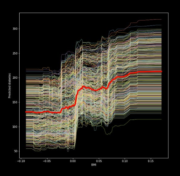
The chart shows that the "bmi," a quantitative indicator of diabetes one year after diagnosis, and our aim have a positive association. The partial dependence plot, represented by the thick red line in the center, illustrates how the average prediction changes as the "bmi" feature is changed.
In order to make sure that the lines for every occurrence in the data begin at the same location, we can additionally center the ICE plot. This eliminates level effects and improves readability of the plot. In the code, we simply need to modify one argument.

icebox.ice_plot(bmi_ice_df, linewidth=.5,  plot_pdp=True, 
         pdp_kwargs={'c': 'blue', 'linewidth': 5}, centered=True, ax=ax1)
ax1.set_ylabel('Predicted diabetes')
ax1.set_xlabel('BMI')

Global justifications:

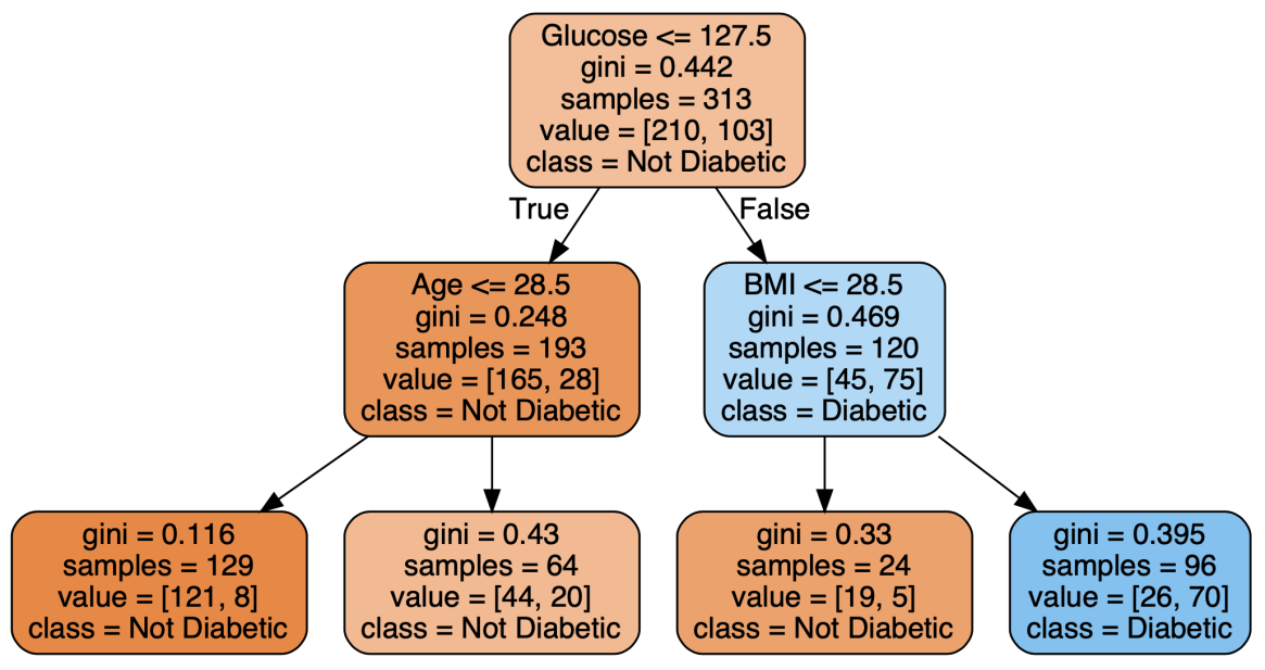
Using the "global surrogate model" is a common method of explaining a black box model's overall behavior. We use our black-box model to generate predictions, that is the purpose. We then use the predictions made by the black-box model and the original features to train a transparent model (imagine a shallow decision tree or linear/logistic regression). Monitoring how closely the surrogate model resembles the black-box model is important, but it's frequently difficult to do so. 

Let's start with getting the predictions after the random forest and building a shallow decision tree.

predictions = clf.predict(X)
dt = DecisionTreeRegressor(random_state = 100, max_depth=3)
dt.fit(X, predictions)

Predicting diabetes Surrogate Model: 

Shapley values in local explanations:

The marginal contribution of each feature, on an instance level, is determined by the Shapley values in relation to the average prediction for the data set. It does well with tabular data, text, and image processing, as well as classification and regression applications. It guarantees a fair distribution of the features' contributions and incorporates every feature for every occurrence.

# explain the model's predictions using SHAP values
# This is the part that can take a while to compute with larger datasets
explainer = shap.TreeExplainer(clf)
shap_values = explainer.shap_values(X)

Final thoughts and future actions:

We discussed what machine learning explainability is and why it should be used (or not). Before getting started on a use case where we applied several techniques using Python and an open data source, we had a quick discussion on the kinds of explanations we can offer. However, this is only the very beginning! The field of XAI is enormous and expanding quickly. Numerous other techniques exist that highlight specific algorithms as well as model-agnostic techniques that apply to any kind of algorithm.